Slurping up SLERP

For work recently, we had to deal with functions on the surface of the sphere. While conceptually simple, this actually introduces more complexity to computations. Even something as simple as distance calculations are now different due to the curvature.

Most of these concepts are really well defined by Wikipedia or other resources. The only qualm I have with the source is the fact that there is no standardization of notation: the usage of $\theta$ and $\varphi$ are almost different and this, frankly, costed me a lot of grief.

However, the concept of shortest point interpolation (so called slerp) between two points on the sphere was really not well explained I think. There is a Scipy implementation, and a short Wikipedia article but both never really discussed the proof of why the formula

\begin{align}
S(p_0, p_1, t) = \frac{\sin((1 – t)\theta)}{\sin \theta} p_0 + \frac{\sin(t\theta)}{\sin(\theta)}p_1
\end{align}

where $\theta = \arccos(p_0 \cdot p_1)$ is actually on the sphere. I was using this for a plotting purpose, so I didn’t care about the “interpolation” aspect, but see this post for a derivation from that point of view.

Let’s quickly give detailed proofs on why this formula works, and to prove that for any $0\le t \le 1$ that we get a point on the sphere that lies on the great circle between the two points $p_0, p_1$. On a sphere of radius 1, $\theta$ is in fact the great circle distance between $p_0$ and $p_1$.

To this end, we have to show that the points defined by slerp is of norm 1, and also lies on the plane defined by the origin, and $p_0, p_1$ (definition of the great circle). This second point is easy to do, we simply have to show that $S(p_0, p_1, t) \cdot (p_0 \times p_1) = 0$ (e.g. the slerp points are orthogonal to the vector which defines the plane). This equality is true due to the simple equaliy $a \cdot (a \times b) = 0$.

Thus the slerp points lies on the plane defined by the great circle, it remains to show that the norm is actually 1. This can be done with just the sine subtraction formula and the usual Pythagorean identity. First note
\begin{align*}
\left\Vert S(p_0, p_1, t) \right\Vert^2 &= \frac{\sin^2((1-t)\theta) + \sin^2(t \theta) + 2 \sin((1-t)\theta) \sin(t\theta) \cos(\theta) } {\sin^2(\theta)}
\end{align*}
by the fact $p_0, p_1$ are norm 1.
Expanding the first term, we have
\begin{align*}
\sin^2((1-t)\theta) = \sin^2(\theta) \cos^2(t\theta) + \cos^2(\theta) \sin^2(t\theta) – 2 \sin(\theta) \cos(\theta) \sin(t\theta) \cos(t\theta).
\end{align*}
and note that the cross term can be expanded using the same sine difference formula
\begin{align*}
2 \sin((1-t)\theta) \sin(t\theta) \cos(\theta) &= 2 \sin(\theta)\cos(\theta)\sin(t\theta)\cos(t\theta) – 2 \cos^2(\theta) \sin^2(t\theta).
\end{align*}
Thus, cancelling the common terms, we have that the numerator is equal to
\begin{align*}
\sin^2(\theta) \cos^2(t\theta) + \cos^2(\theta) \sin^2(t\theta) + \sin^2(t \theta)- 2 \cos^2(\theta) \sin^2(\theta) = \\
\sin^2(\theta) \cos^2(t\theta) + (\cos^2(\theta) +1- 2 \cos^2(\theta)) \sin^2(t\theta) = \\
\sin^2(\theta) \cos^2(t\theta) + (\sin^2(\theta)) \sin^2(t\theta) = \sin^2(\theta)
\end{align*}
which equals the denominator.

My (Not-So-Successful) Quest to Conquer the NYT Connections Game with Word2Vec

The New York Times’ Connections game: a fairly simple puzzle that has been rising in popularity. The objective? Find four groups for four within a larger sample of sixteen total words such that each subgroup has an overarching theme.

I thought this would be fairly easy to solve with some simple usage of word embedding and K-means clustering. After all, if it can figure out king – man + woman = queen, then surely it can figure out that these are all sandwich ingredients. There are enough models out there for topic modelling that it was easy to install a model in under 1 minute, and I just used a simple K-means.

However, I quickly ran into problems. The most major is the fact that K-means doesn’t always give four groups of four. Seeing as this was the case, I switched to a constrained K-means algorithm. Another thing I noticed is that the word embedding probably doesn’t account for the fact that repetition might be used (e.g. ‘tom tom’ rather than ‘tom’).

It’s curious to wonder what a better approach would be, as spending some 2 hours on this little question has proved to be not as fruitful, even for some relatively simple puzzles. Maybe a contextual embedding is needed, rather than just a GLOVE word2vec model.

I also thought a more curated, greedy algorithm might work rather than K-means. Take the two most similar words, and assume they must be a group. Average the two word vectors then find the next word from the now reduced list. I gave this a whack, but also didn’t turn out too well…

… maybe this is a more difficult puzzle than I originally thought.

Nevertheless, below is some sample code:


import gensim.downloader
from sklearn.metrics.pairwise import cosine_similarity
from k_means_constrained import KMeansConstrained

words = [
    'plastic', 'foil', 'cellophane', 'lumber',
    'organism', 'harpoon', 'trudge', 'limber',
    'stomp', 'elastic', 'glove', 'bassinet',
    'mask', 'plod', 'jacket', 'supple'
]

# Load model
model = gensim.downloader.load('glove-wiki-gigaword-300')

# Generate similarity matrix
word_vectors = [
    model[word] for word in words # We assume all words exist in corpus
]
sim_matrix = cosine_similarity(word_vectors)

clf = KMeansConstrained(n_clusters=4, size_min=4, size_max=4, random_state=0)
clf.fit_predict(sim_matrix)

print([x for _, x in sorted(zip(clf.labels_, words))])
print(sorted(clf.labels_))

Transformers

Title Generator

The point of this post is pretty straightforward: apply an encoder-decoder Transformer model to yet another text generation task. The problem at hand is to generate a title given the abstract of a scientific paper.

I’m trying to figure out how to have Jupyter notebooks on WordPress; the export to HTML seems fine, but it’s hard to run. This notebook can be downloaded from here.

Load and process data

We will use the Arxiv dataset which consists of 1.7 million articles with parsed information. The dataset is quite large at over 3GB, and we’ll be only interested in using a small subset. Thus, we first process this by only parsing out a set number of articles’ title and abstract which are from a specific scientific field.

We use read_json from pandas to process the data file, remove all other columns and create a single DataFrame after removing leading/trailing white space and newline characters.

In [1]:
# Pytorch
import torch
from torch.utils.data import Dataset, DataLoader, random_split
from torch.nn.utils.rnn import pad_sequence
from torch import nn
import torch.optim as optim

import pandas as pd
from tqdm.notebook import tqdm
from matplotlib import pyplot as plt
import math
import numpy as np
In [2]:
# Let's set some variables for the data processing part
TOTAL_ARTICLES = 300000
FIELD = 'astro'
In [3]:
# We read a few lines at a time; note that if `chunksize` is none, the whole thing is read to memory
chunks = pd.read_json('arxiv-metadata-oai-snapshot.json', lines=True, chunksize=2048)

astro_dfs = []
num_articles = 0
for entries in tqdm(chunks):
    # We find all articles of a certain field, and then discard the rest of the columns
    astro_dfs.append(
        entries[entries['categories'].str.contains(FIELD)].drop(
            ['id', 'submitter', 'authors', 'comments', 'journal-ref', 'doi',
            'report-no', 'categories', 'license', 'versions',
            'update_date', 'authors_parsed'], axis='columns'
        )
    )
    num_articles += len(astro_dfs[-1])

    # We stop once we have enough of a dataset
    if num_articles > TOTAL_ARTICLES:
        break
In [4]:
# Make one dataframe, and we remove the \n in the text
data_df = pd.concat(astro_dfs, ignore_index=True)
data_df = data_df.replace(r'\n',' ', regex=True)
data_df['title'] = data_df['title'].str.strip()
data_df['abstract'] = data_df['abstract'].str.strip()
In [5]:
data_df
Out[5]:
title abstract
0 The Spitzer c2d Survey of Large, Nearby, Inste… We discuss the results from the combined IRAC …
1 Spectroscopic Observations of the Intermediate… Results from spectroscopic observations of the…
2 ALMA as the ideal probe of the solar chromosphere The very nature of the solar chromosphere, its…
3 Astrophysical gyrokinetics: kinetic and fluid … We present a theoretical framework for plasma …
4 Inference on white dwarf binary systems using … We report on the analysis of selected single s…
301116 The imprint of massive black hole formation mo… The formation, merging, and accretion history …
301117 Resolving the Stellar Populations in the Circu… We investigate the stellar populations in the …
301118 UVES – VLT High Resolution Spectroscopy of GRB… We present early time, high resolution spectro…
301119 Far-Infrared detection of H2D+ toward Sgr B2 We report on the first far-IR detection of H2D…
301120 DE CVn: A bright, eclipsing red dwarf – white … Close white dwarf – red dwarf binaries must ha…

301121 rows × 2 columns

Tokenize Data

With the text in an easy to manipulate DataFrame, we have to convert the text to a numerical representation. Here, we use pre-trained tokenizers from Huggingface rather than build/train our own. Roughly speaking, a tokenizer takes a word and maps it to an integer. However, often times, modern tokenizers “understand” parts of words and would also parse out the prefix/suffix of a word too.

For simplicity, we’re only going to use 384 tokens for the abstract and 64 tokens for the title, and discard the rest. This is usually not a problem for the title (as it is quite short), but will generally truncate the abstract. However, judging from the box plot, the number of tokens seem fine. Ideally, our model would incorporate the full abstract, however the amount of compute power needed will be a lot larger due to the quadratic scaling of the transformers.

In [9]:
from transformers import AutoTokenizer
checkpoint = "bert-base-uncased"
tokenizer = AutoTokenizer.from_pretrained(checkpoint)

# This is fairly slow,
data_tokenized = pd.DataFrame()
data_tokenized['abstract'] = data_df['abstract'].apply(
    lambda w: torch.Tensor(tokenizer(w, truncation=True, max_length=256+128)['input_ids']).int()
)
data_tokenized['title'] = data_df['title'].apply(
    lambda w: torch.Tensor(tokenizer(w, truncation=True, max_length=64)['input_ids']).int()
)
In [13]:
plt.boxplot(data_tokenized['abstract'].str.len(), vert=False)
plt.boxplot(data_tokenized['title'].str.len(), vert=False)
plt.show()

Data Loader

With the data in a numerical form, we can start loading them into PyTorch Dataset/DataLoader objects. This will help facilitate easier training.

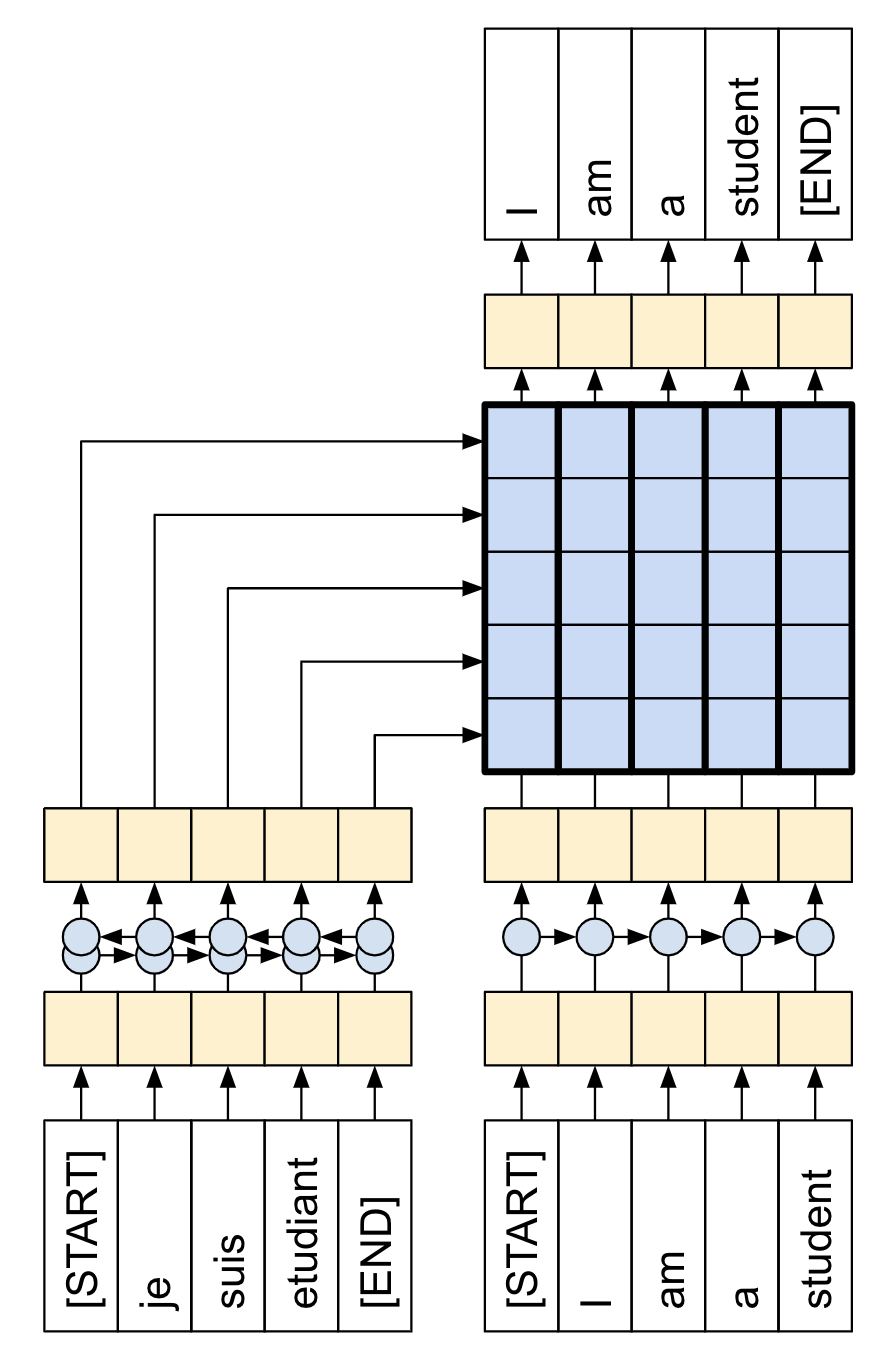
Here, we note that we want to generate datasets which are applicable for “teacher forcing” learning. In our case, we want to deduce a sequence $(x_1, x_2, \ldots, x_{n+1})$ from $(x_0, \ldots, x_n)$. See figure (source) below. In our case the French corresponds to the abstract while the English is the title. This means that we would need to shift the titles by 1 in the collate_fn function for the DataLoader. We also take the opportunity here to perform the train/validation split.
drawing

In [14]:
class ArxivDataset(Dataset):
    def __init__(self, dataframe):
        self.df = dataframe

    def __len__(self):
        return len(self.df)

    def __getitem__(self, idx):
        """
        Returns abstract, then title
        """
        return self.df.iloc[idx, 0], self.df.iloc[idx, 1]

def pad_collate(batch):
    my_abstracts, my_titles = zip(*batch)

    # Pad sequence together, with 0 added
    my_abstracts = pad_sequence(my_abstracts, batch_first=True)
    my_titles = pad_sequence(my_titles, batch_first=True)

    # For teacher training, need to shift
    titles_inp = my_titles[:, 0:-1]
    titles_lab = my_titles[:, 1:]

    return (my_abstracts, titles_inp), titles_lab
In [15]:
dataset = ArxivDataset(data_tokenized)

train_size = int(0.8 * len(dataset))
test_size = len(dataset) - train_size
train_dataset, test_dataset = random_split(dataset, [train_size, test_size])

train_dataloader = DataLoader(train_dataset, batch_size=256+64, shuffle=True, collate_fn=pad_collate)
test_dataloader = DataLoader(test_dataset, batch_size=256+64, shuffle=True, collate_fn=pad_collate)
print(len(train_dataloader), len(test_dataloader))
753 189

Transformer model

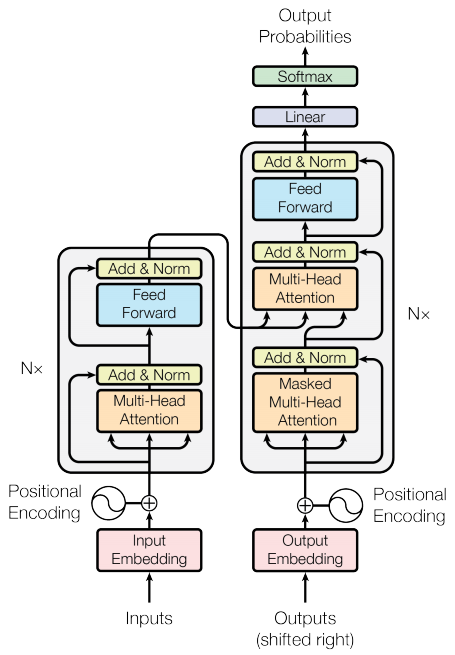
Note that this is not intended as a tutorial for how to build a transformer, and we will gloss over most details. Roughly speaking, a transformer is a sequence-to-sequence model which supplies the probability distribution of the next element. First the abstract is embedded in some latent space by the encoder, which is then use by the decoder to condition for the prediction.

It is similar to RNNs, however, the main technique for a transformer is the attention mechanism, which is implemented in PyTorch. This allows transformers, in theory, to couple far ranging words with each other rather easily as a quadratic 1-to-1 comparison is done between every element in the sequence. With this extra $n^2$ expense, comes at a benefit of it seemingly able to learn languages very well.

PyTorch in theory has a Transformer module but it is not well documented. We will perform a quick and dirty implementation here. For more details, we refer to a great tutorial here. The schematics below should serve as enough of a guideline for the code below.

In [12]:
device = torch.device('cuda' if torch.cuda.is_available() else 'cpu')

Positional Embedding

In [4]:
class PositionalEncoding(nn.Module):
    def __init__(self, d_model, max_len=5000):
        """
        Inputs
            d_model - Hidden dimensionality of the input.
            max_len - Maximum length of a sequence to expect.
        """
        super().__init__()

        # Create matrix of [SeqLen, HiddenDim] representing the positional encoding for max_len inputs
        pe = torch.zeros(max_len, d_model)
        position = torch.arange(0, max_len, dtype=torch.float).unsqueeze(1)
        div_term = torch.exp(torch.arange(0, d_model, 2).float() * (-math.log(10000.0) / d_model))
        pe[:, 0::2] = torch.sin(position * div_term)
        pe[:, 1::2] = torch.cos(position * div_term)
        pe = pe.unsqueeze(0)

        # register_buffer => Tensor which is not a parameter, but should be part of the modules state.
        # Used for tensors that need to be on the same device as the module.
        # persistent=False tells PyTorch to not add the buffer to the state dict (e.g. when we save the model)
        self.register_buffer('pe', pe, persistent=False)

    def forward(self, x):
        x = x + self.pe[:, :x.size(1)]
        return x

Encoder Block

This just consists of a multihead attention (essentially a few attentions concat-ed together), and a feed-forward NN.

In [5]:
class EncoderBlock(nn.Module):
    def __init__(self, input_dim, num_heads, dim_feedforward, dropout=0.1):
        super().__init__()

        # Attention layer
        self.self_attn = nn.MultiheadAttention(
            embed_dim=input_dim,
            num_heads=num_heads, batch_first=True
        )

        # Two-layer MLP
        self.linear_net = nn.Sequential(
            nn.Linear(input_dim, dim_feedforward),
            nn.Dropout(dropout),
            nn.ReLU(inplace=True),
            nn.Linear(dim_feedforward, input_dim)
        )

        # Layers to apply in between the main layers
        self.norm1 = nn.LayerNorm(input_dim)
        self.norm2 = nn.LayerNorm(input_dim)
        self.dropout = nn.Dropout(dropout)

    def forward(self, x):
        # Attention part
        attn_out, _ = self.self_attn(x, x, x)
        x = x + attn_out
        x = self.norm1(x)

        # MLP part
        linear_out = self.linear_net(x)
        x = x + self.dropout(linear_out)
        x = self.norm2(x)

        return x

class EncoderLayers(nn.Module):
    def __init__(self, num_layers, **encoder_args):
        super().__init__()
        self.layers = nn.ModuleList([EncoderBlock(**encoder_args) for _ in range(num_layers)])

    def forward(self, x):
        for l in self.layers:
            x = l(x)
        return x

Decoder

A decoder layer consists of a causal attention, cross-attention from the decoder, and a final MLP.

In [6]:
# From PyTorch source
def _generate_square_subsequent_mask(
        sz: int,
        dtype: torch.dtype = torch.get_default_dtype(),
):
    r"""Generate a square causal mask for the sequence. The masked positions are filled with float('-inf').
        Unmasked positions are filled with float(0.0).
    """
    return torch.triu(
        torch.full((sz, sz), float('-inf'), dtype=dtype, device=device),
        diagonal=1,
    )


class DecoderBlock(nn.Module):
    def __init__(self, input_dim, num_heads, dim_feedforward, dropout=0.1):
        super().__init__()

        # Attention layers
        self.causal_self_attn = nn.MultiheadAttention(
            embed_dim=input_dim,
            num_heads=num_heads, dropout=dropout, batch_first=True
        )
        self.cross_attn = nn.MultiheadAttention(
            embed_dim=input_dim,
            num_heads=num_heads, dropout=dropout, batch_first=True,
        )

        # Two-layer MLP
        self.linear_net = nn.Sequential(
            nn.Linear(input_dim, dim_feedforward),
            nn.Dropout(dropout),
            nn.ReLU(inplace=True),
            nn.Linear(dim_feedforward, input_dim)
        )

        # Layers to apply in between the main layers
        self.norm1 = nn.LayerNorm(input_dim)
        self.norm2 = nn.LayerNorm(input_dim)
        self.norm3 = nn.LayerNorm(input_dim)
        self.dropout = nn.Dropout(dropout)

    def forward(self, x, context):
        # Causal; create mask
        mask = _generate_square_subsequent_mask(x.shape[1])
        attn_out, _ = self.causal_self_attn(
            x, x, x, attn_mask=mask, is_causal=True
        )
        x = x + attn_out
        x = self.norm1(x)

        # Cross attention
        attn_out, _ = self.cross_attn(
            x, context, context,
        )
        x = x + attn_out
        x = self.norm2(x)

        # MLP
        linear_out = self.linear_net(x)
        x = x + self.dropout(linear_out)
        x = self.norm3(x)

        return x

class DecoderLayers(nn.Module):
    def __init__(self, num_layers, **decoder_args):
        super().__init__()
        self.layers = nn.ModuleList([DecoderBlock(**decoder_args) for _ in range(num_layers)])
    def forward(self, title, abstract):
        for l in self.layers:
            title = l(x=title, context=abstract)
        return title

Full Model

The transformer full model is simply the above two blocks, alongside some embeddings and a final classifier layer.

In [7]:
class Transformer(nn.Module):
    def __init__(self, num_layers, model_dim, num_heads, dff,
               vocab_size, dropout=0.2):
        super().__init__()

        # Needed for scaling
        self.model_dim = model_dim

        # Embedding
        self.embedding = nn.Embedding(
            num_embeddings=vocab_size, embedding_dim=model_dim
        )

        # Positional
        self.positional_encoding = PositionalEncoding(d_model=model_dim)

        self.encoder = EncoderLayers(
            num_layers=num_layers, input_dim=model_dim, num_heads=num_heads, dim_feedforward=dff, dropout=dropout
        )
        self.decoder = DecoderLayers(
            num_layers=num_layers, input_dim=model_dim, num_heads=num_heads, dim_feedforward=dff, dropout=dropout
        )

        # Final layer which maps to "probabilities" in the token space
        self.ff = nn.Linear(model_dim, vocab_size)

    def forward(self, title, abstract):
        # Apply embedding and position
        title       = self.embedding(title) * math.sqrt(self.model_dim)
        abstract    = self.embedding(abstract) * math.sqrt(self.model_dim)

        # Add positional
        title       = self.positional_encoding(title)
        abstract    = self.positional_encoding(abstract)

        # Apply encoder than decoder
        abstract    = self.encoder(abstract)
        title       = self.decoder(title, abstract)

        return self.ff(title)

Training

There are heuristics for training transformers; one of them is that a warmup should be used. We use the cosine warmup as detailed in the tutorial linked above. Another small caveat is that for the cross entropy loss, to ignore the index 0 (where padding occurred), as we don’t want the optimizer to optimize over dummy data.

Besides the two notes above, the below should be fairly similar to the usual training procedure.

In [22]:
class CosineWarmupScheduler(optim.lr_scheduler._LRScheduler):

    def __init__(self, optimizer, warmup, max_iters):
        self.warmup = warmup
        self.max_num_iters = max_iters
        super().__init__(optimizer)

    def get_lr(self):
        lr_factor = self.get_lr_factor(epoch=self.last_epoch)
        return [base_lr * lr_factor for base_lr in self.base_lrs]

    def get_lr_factor(self, epoch):
        lr_factor = 0.5 * (1 + np.cos(np.pi * epoch / self.max_num_iters))
        if epoch <= self.warmup:
            lr_factor *= epoch * 1.0 / self.warmup
        return lr_factor
In [33]:
def train(dataloader, my_model, my_criterion, my_optimizer, my_scheduler, my_epoch, interval=500):
    """
    Training loop for one epoch
    """
    losses = []
    model.train()
    for batch_idx, ((abstract, title_inp), title_lab) in enumerate(dataloader):
        # Move to GPU
        abstract = abstract.to(device)
        title_inp = title_inp.to(device)
        title_lab = title_lab.type(torch.long)
        title_lab = title_lab.to(device)

        pred = my_model(title_inp, abstract)
        loss = my_criterion(
            pred.reshape(-1, MAX_VOCAB), title_lab.reshape(-1)
        )

        my_optimizer.zero_grad()
        loss.backward()
        torch.nn.utils.clip_grad_norm_(my_model.parameters(), 5)
        my_optimizer.step()
        my_scheduler.step()

        losses.append(loss.item())

        if batch_idx 
            print(f'Epoch {my_epoch} |  {batch_idx / len(dataloader) * 100:.1f}

    return losses

def test(dataloader, my_model, my_criterion, my_epoch):
    """
    Training loop for one epoch
    """
    val_loss = 0
    val_acc = 0
    val_total = 0
    model.eval()
    with torch.no_grad():
        for _, ((abstract, title_inp), title_lab) in enumerate(dataloader):
            # Move to GPU
            abstract = abstract.to(device)
            title_inp = title_inp.to(device)
            title_lab = title_lab.type(torch.long)
            title_lab = title_lab.to(device)
            title_lab = title_lab.reshape(-1)

            pred = my_model(title_inp, abstract)
            pred = pred.reshape(-1, MAX_VOCAB)
            loss = my_criterion(
                pred, title_lab
            )

            val_loss += loss.item()

            # Count number of correct predictions
            pred = torch.argmax(pred, dim=1, keepdim=True)
            title_lab = title_lab.reshape_as(pred)
            val_acc += torch.count_nonzero(pred.eq(title_lab) * (title_lab != 0)).item()
            val_total += torch.count_nonzero(title_lab).item()

    val_loss /= len(dataloader)
    val_acc /= val_total

    print(f'Epoch {my_epoch} | Validation Loss: {val_loss:.2f} | Validation Accuracy: {val_acc * 100:.1f}

    return val_loss, val_acc
In [34]:
epochs = 40
lr = 5e-5
MAX_VOCAB = len(tokenizer)

model = Transformer(num_layers=6, model_dim=256, num_heads=8, dff=2056, vocab_size=MAX_VOCAB).to(device)

print(f'Using {device}')

optimizer = optim.Adam(model.parameters(), lr=lr)
scheduler = CosineWarmupScheduler(optimizer, 5000, MAX_VOCAB * epochs)
criterion = nn.CrossEntropyLoss(ignore_index=0)

train_loss = []
val_loss = []
val_acc = []
model.train()
for epoch in range(1, epochs + 1):
    e_loss = train(train_dataloader, model, criterion, optimizer, scheduler, epoch, interval=100)
    train_loss += e_loss
    v_loss, v_acc = test(test_dataloader, model, criterion, epoch)

    val_loss.append(v_loss)
    val_acc.append(v_acc)
Using cuda
Epoch 1 |  0.0
Epoch 1 |  13.3
Epoch 1 |  26.6
Epoch 1 |  39.8
Epoch 1 |  53.1
Epoch 1 |  66.4
...
Epoch 40 |  39.8
Epoch 40 |  53.1
Epoch 40 |  66.4
Epoch 40 |  79.7
Epoch 40 |  93.0
Epoch 40 | Validation Loss: 2.61 | Validation Accuracy: 48.9
In [35]:
# Save model
state_dict = model.state_dict()
torch.save(state_dict, "large_model_v2.pt")

# Plot loss and stuff
fig, ax1 = plt.subplots()

ax1.plot(train_loss)
ax1.set_xlabel('Batch num')
ax1.set_ylabel('X-entropy Loss')
ax1.plot(np.arange(1, len(val_loss) + 1) * len(train_dataloader) ,val_loss)
ax1.plot([], [], 'r', label = 'temp') # Just for legends; hack

ax2 = ax1.twinx()
ax2.set_ylabel('Validation Accuracy')
ax2.plot(np.arange(1, len(val_loss) + 1) * len(train_dataloader),
         np.array(val_acc) * 100, 'r')
fig.tight_layout()
ax1.legend(['Train loss', 'Test loss', 'Test acc'])
plt.savefig('loss_good.png')

plt.show()

Inference

The above training does take awhile on an A100, and it’s not even the best results. With additional tweaking and modifications, we can probably do a lot better. In addition, we should probably look at a more specific field rather than “astro” as a whole. However, let’s move on to writing the inference.

To build a generator is easy: we start with $(x_0)$ where $x_0$ is the start token and repeatedly query the model conditioned on the abstract input. For example, the first token will be given by $x_0 \to x_1$, which we then pass in $(x_0, x_1) \to (x_1, x_2)$ and iterate. We stop once we encounter a stop token or if it reaches the number of max tokens.

In [15]:
# Reimport so I can load the model in a future date
from transformers import AutoTokenizer
checkpoint = "bert-base-uncased"
tokenizer = AutoTokenizer.from_pretrained(checkpoint)

MAX_VOCAB = len(tokenizer)
model = Transformer(num_layers=6, model_dim=256, num_heads=8, dff=2056, vocab_size=MAX_VOCAB).to(device)
model.load_state_dict(torch.load( "large_model_v2.pt"))
model.eval()
print('Loaded model')
Loaded model
In [16]:
class TitleGenerator(nn.Module):
    def __init__(self, transformer_model: nn.Module, my_tokenizer):
        super().__init__()

        self.model = transformer_model
        self.tokenizer = my_tokenizer

    def forward(self, x: str):
        """
        Given an abstract, it should query the transformer

        :param x: Should be the abstract
        :return:
        """
        # Get tokenized
        tokenized = self.tokenizer(x, return_tensors='pt')['input_ids']
        tokenized = tokenized.to(device)
        output = torch.tensor([[101]]).to(device)
        self.model.eval()
        with torch.no_grad():
            for i in range(128):
                probs = self.model(output, tokenized)
                pred = probs.argmax(dim=2)
                output = torch.cat((output, pred[0, -1].view(1, 1)), dim=1)
                if output[0, -1] == 102:
                    break

        return self.tokenizer.decode(output[0])
In [17]:
generate = TitleGenerator(model, tokenizer)
generate('We discuss the combined IRAC/MIPS c2d Spitzer Legacy observations of the Serpens star-forming region. We describe criteria for isolating bona fide YSOs from the extensive background of extragalactic objects.')
Out[17]:
'[CLS] extragalactic star - forming regions from spitzer irac observations of the irac - irac region [SEP]'
In [18]:
generate('We explore the reach of analytical models at one-loop in Perturbation Theory (PT) to accurately describe measurements of the galaxy power spectrum from numerical simulations in redshift space. We consider the validity range in terms of three different diagnostics: 1) the goodness of fit; 2) a figure-of-bias quantifying the error in recovering the fiducial value of a cosmological parameter; 3) an internal consistency check of the theoretical model quantifying the running of the model parameters with the scale cut.')
Out[18]:
'[CLS] the effect of loop corrections on the power spectrum of galaxy power spectra in the large - scale structure of the universe [SEP]'
In [20]:
generate('There has been a discussion for many years on whether the disc in the Milky Way extends down to low metallicity. We aim to address the question by employing a large sample of giant stars with radial velocities and homogeneous metallicities based on the Gaia DR3 XP spectra. We study the 3D velocity distribution of stars in various metallicity ranges, including the very-metal poor regime (VMP, [M/H] <−2.0). We find that a clear disc population starts to emerge only around [M/H] ∼−1.3, and is not visible for [M/H] <−1.6. Using Gaussian Mixture Modeling (GMM), we show that there are two halo populations in the VMP regime: one stationary and one with a net prograde rotation of ∼80km/s. In this low-metallicity range, we are able to place constraints on the contribution of a rotation-supported disc sub-population to a maximum of ∼3%. We compare our results to previous claims of discy VMP stars in both observations and simulations and find that having a prograde halo component could explain most of these. ')
Out[20]:
'[CLS] the metallicity distribution of the milky way disc with gaia dr3 [SEP]'

np.vectorize quirk

I was being lazy, and had to code up a piecewise function. Rather than use the proper array tools, I used np.vectorize instead but somehow got weird results:

import numpy as np

def f(x):
if x < .5:
return 1
else:
return .4

points = np.linspace(0, 1, 5)

points_flipped = np.flip(points)

vec_f = np.vectorize(f)

print(vec_f(points))

print(vec_f(points_flipped))

returns [1 1 0 0 0]
[0.4 0.4 0.4 1. 1. ]

Tuorns out np.vectorize has the property that

The output type is determined by evaluating the first element of the input, unless it is specified

Took me a minute to figure this out. RTFM.

Calvin’s Interesting Question

Calvin and Hobbes (October 19, 1989)

Given a set of positive integers $\{q_i\}_{i=1}^n$, describe the set $s_t \in S$ of positive integers such that there exists only one linear combination of $\sum_{i=1}^n a_i q_i = s_t$.

In the comic above, it’s pretty obvious with the amount of money given, that Calvin was hoping to get four “D”s. In fact, all integers from 1 to 9 can only be expressed in one permutation.

A satisfying answer to all sets of integers might be less trivial.

Putnam 2022 A1

Determine all ordered pairs of real numbers $(a, b)$ such that the line $y = ax + b$ intersects the curve $y = \ln(1 + x^2)$ in exactly one point.

I really liked this problem, and thought it makes for a good “research” problem for calculus classes. For notation purposes, let $g(x) = \ln(1 + x^2)$. The following is also very sketch-like, and conversational. We first note that logarithmic curve is even, and we can simply consider $a \ge 0$, since $y = -ax + b$ will have the same number of intersection points. Simply looking at the graph, it’s clear that $(a, b) = (0, 0)$ is such a solution, and for fixed $a = 0$, that no other $y$-intercept will work.

Intuitively, for large enough slope, a line will also only intersect $g(x)$ at one point, no matter the intercept since it “outgrows” the log. We can formalize this by noting that $g'(x) = \frac{2x}{1 + x^2}$ with

  1. $\lim_{x\to \pm \infty} g'(x) = 0$,
  2. $g'(0) = 0, g'(1) = 1$
  3. $g'(x) \le 1$ by trivial inequality.

Assume not, then there exists two or more zeros for the function $g(x) – (ax + b)$. By the mean value theorem, then there would exist a point $c$ such that $g'(c) – a = 0$, which cannot happen since $|g'(c)| \le |a|$.

Now, we need to examine the region where $1 > a > 0$. For $b > 0$, if the $y$-intercept is large enough then the logarithmic growth will not catch up with the linear growth. To find this “large enough” intercept, we set simply find the line where it intersects $g(x)$; this will occur where the derivatives equal.

Solving $g'(x) = a$, we have $\frac{2x}{1 + x^2} = a \implies x^*_{\pm} = \frac{1 \pm \sqrt{1 – a^2}}{a}$. The intersection $b$ will be $ax^*_{+} + b = \ln(1 + (x^*_p)^2) \implies b = \ln(1 + (x^*_p)^2) – ax^*_p$, hence any $b > \ln(1 + ((x^*_p)^2) – ax^*_p$ suffices.

On the other hand, the root $x^*_{-}$ corresponds to the cases where $b < 0$ where the line “ducks” underneath first before intersecting the log curve, and hence any $b < \ln(1 + (x^*_m)^2) – ax^*_m$ will work.

Finally,the case of $a = 1$ is left as an exercise because this is too long.

Interpolation in Tensorflow

I recently had to interpolate some data in the setting of training some machine learning code, coded in Tensorflow. It turns out that the interpolator doesn’t work with the compiled Tensorflow functions, which is usually recommended for faster execution.
This is quite annoying, but has a simple solution using the

numpy_function

in Tensorflow.

import tensorflow as tf
import numpy as np
from scipy.interpolate import NearestNDInterpolator

x = np.linspace(0, 10, 10)
y = np.linspace(0, 10, 10)
z = np.sin(x + y)
interp = NearestNDInterpolator(list(zip(x, y)), z)
points = tf.constant([[1, 2],
[3, 4],
[5, 6]], dtype=tf.float64)
@tf.function
def test(x):
return interp(x)
@tf.function
def test_2(x):
return tf.numpy_function(interp, inp=[x], Tout=tf.float64)
print(test_2(points)) # Works
print(test(points)) # Doesn't work

Putnam 2020 A2

For $k$ a non-negative integer, evaluate
\begin{align*}
\sum_{j=0}^k 2^{k-j} \binom{k +j}{j}.
\end{align*}

Apparently, I only know how to do induction anymore now but this problem is straightforward using it. We suppose the inductive hypothesis, and assume that for a fixed $k$ that
\begin{align*}
\sum_{j=0}^k 2^{k-j} \binom{k +j}{j} = 2^{2k}.
\end{align*}
We will proceed to show
\begin{align*}
\sum_{j=0}^{k + 1} 2^{k + 1-j} \binom{k + 1 +j}{j} = 2^{2k + 2}.
\end{align*}

By a simple binomial identity, we have
\begin{align*}
\sum_{j=0}^{k + 1} 2^{k + 1-j} \binom{k + 1 +j}{j} &= \sum_{j=0}^{k + 1} 2^{k + 1-j} \binom{k+j}{j} + \sum_{j=0}^{k + 1} 2^{k + 1-j} \binom{k +j}{j – 1}.
\end{align*}
Let $A$, $B$ be the first and second term respectively on the right hand side, then
\begin{align*}
A &= 2\sum_{j=0}^{k} 2^{k-j} \binom{k+j}{j} + \binom{2k + 1}{k+1} \\
&= 2^{2k + 1} + \binom{2k + 1}{k+1}.
\end{align*}
For the other term,
\begin{align*}
B &= \sum_{j=1}^{k + 1} 2^{k + 1-j} \binom{k +j}{j – 1} \\
&= \sum_{j=0}^{k} 2^{k-j} \binom{k +1 +j}{j} \\
&= \frac{1}{2} \sum_{j=0}^{k + 1} 2^{k + 1-j} \binom{k +1 +j}{j} – \frac{1}{2} \binom{2k + 2}{k + 1}.
\end{align*}
Thus, we rearranging, we have our result
\begin{align*}
\frac{1}{2}\sum_{j=0}^{k + 1} 2^{k + 1-j} \binom{k + 1 +j}{j} &= 2^{2k+1} + \binom{2k + 1}{k+1} – \frac{1}{2} \binom{2k + 2}{k + 1} \\
&= 2^{2k+1}.
\end{align*}

Saddle Point Property

I felt dumb while trying to derive this, so here it is. Sourced from page 129 of Braess FEM textbook.

Let $X, M$ be two Hilbert spaces, and $a: X \times X \to \mathbb{R}, \, b: X \times M \to \mathbb{R}$ continuous bilinear forms.
Assume that $a$ is symmetric and that $a(u, u) \ge 0$ for all $u \in X$.
Let $f \in X’, g \in M’$ and let
\begin{align*}
\mathcal{L}(v, \mu) &= \frac{1}{2}a(v, v) – \langle f, v \rangle + (b(v, \mu) – \langle g, \mu\rangle)
\end{align*}
which is simply the Lagrangian of a constrained minimization problem.
Assume that $(u, \lambda)$ satisfies
\begin{align}
a(u, v) + b(v, \lambda) &= \langle f, v \rangle \qquad &\forall v \in X, \\
b(u, \mu) &= \langle g, \mu \rangle \qquad &\forall \mu \in M,
\end{align}
then one has the saddle point property
\begin{align*}
\mathcal{L}(u, \mu) \le \mathcal{L}(u, \lambda) \le \mathcal{L}(v, \lambda) \qquad \forall (v, \mu) \in X \times M.
\end{align*}

The first inequality is actually an equality by noting that $\mathcal{L}(u, \mu) = \frac{1}{2}a(u, u) – \langle f, u \rangle= \mathcal{L}(u, \lambda)$ by using (2).
For the other inequality, let $v = u + w$, then
\begin{align*}
\mathcal{L}(v, \lambda) = \mathcal{L}(u + w, \lambda) &= \frac{1}{2}a(u + w, u + w) – \langle f, u + w \rangle + (b(u + w, \lambda) – \langle g, \lambda\rangle) \\
&= \mathcal{L}(u, \lambda) + \frac{1}{2}a(w, w) – \langle f, w \rangle + a(u, w) + b(w, \lambda) \\
&= \mathcal{L}(u, \lambda) + \frac{1}{2}a(w, w) \ge\mathcal{L}(u, \lambda)
\end{align*}
where (1) and (2) are used.

A fixed order double integral

I have a good example where copying code straight from Stackoverflow is a terrible idea. Consider a simple rectangle $[0, 1] \times [0, 2]$ which we want to perform a double integral over. Of course, there’s the classic way to use scipy’s $\texttt{dblquad}$

In [1]:
from scipy.integrate import dblquad

def f(x, y): 
    return x + 2 * y

dblquad(lambda y, x: f(x, y), 0, 1, lambda x: 0, lambda x: 2)[0]
Out[1]:
5.0

This above is all and nice, but $\texttt{dblquad}$ is very accurate, and hence slow. What if we don’t need that level of accuracy? We can try to use the $\texttt{fixed_quad}$ function in scipy. Here’s a Stackoverflow question about the exact same thing, with some sample code.

Let’s copy its code and test it. It seems to work:

In [2]:
from scipy.integrate import fixed_quad

fixed_quad(lambda x: fixed_quad(f, 0, 1, args=(x, ), n=5)[0], 0, 2, n=5)[0]
Out[2]:
5.000000000000001

Of course, we have very fast speed up, at least on my laptop

In [3]:

10000 loops, best of 3: 39.3 µs per loop
In [4]:

1000 loops, best of 3: 261 µs per loop

Seems to work well right? It’s too bad it fails for very simple cases…

In [5]:
def g(x, y): 
    return x * y

print(dblquad(lambda y, x: g(x, y), 0, 1, lambda x: 0, lambda x: 2)[0])
print(fixed_quad(lambda x: fixed_quad(g, 0, 1, args=(x, ), n=5)[0], 0, 2, n=5)[0])
0.9999999999999999
1.333333333333333

Ah, what’s going wrong? Turns out it has to deal with the way $\texttt{fixed_quad}$ deals with the array. It doesn’t really evaluate the tensor product of the quadrature points, but rather along some subset of it.

A better implementation is just to rewrite the code myself (or to use something like quadpy):

In [6]:
from scipy.special import roots_legendre
import numpy as np
roots, weights = roots_legendre(5)

def dbl_integral(func, left: int, right: int, bottom: int, top: int):
    """
    Calculates double integral \int_c^d \int_a^b f(x, y) dx dy.
    """
    x = (right - left) * (roots + 1) / 2.0 + left

    y = (top - bottom) * (roots + 1) / 2.0 + bottom

    total = 0
    for index_i, i in enumerate(x):
        # The first ones_like(y) is to ensure we obtain a vector for some of my usages... 
        total += np.dot(np.ones_like(y) * func(i, y) * weights[index_i], weights)

    return (top - bottom) * (right - left) / 4 * total
In [7]:
print(dblquad(lambda y, x: f(x, y), 0, 1, lambda x: 0, lambda x: 2)[0])
print(fixed_quad(lambda x: fixed_quad(f, 0, 1, args=(x, ), n=5)[0], 0, 2, n=5)[0])
print(dbl_integral(f, 0, 1, 0, 2))

print(dblquad(lambda y, x: g(x, y), 0, 1, lambda x: 0, lambda x: 2)[0])
print(fixed_quad(lambda x: fixed_quad(g, 0, 1, args=(x, ), n=5)[0], 0, 2, n=5)[0])
print(dbl_integral(g, 0, 1, 0, 2))
5.0
5.000000000000001
5.0
0.9999999999999999
1.333333333333333
1.0

And we also maintain the speed (though not as fast but it’s not hard to write above in einsum or optimize it a bit more), assuming we precalculate the weights and roots:

In [8]:


1000 loops, best of 3: 246 µs per loop
10000 loops, best of 3: 38.1 µs per loop
10000 loops, best of 3: 74.1 µs per loop