My adviser told me about this meshing of a cube (or any hexahedral) into 6 different tetrahedrons which is easy to draw. For the sake of exposition, we will consider the cube $(-1,1)^3$ The procedure is as follows:
- Draw a diagonal from $(-1,-1, -1)$ to $(1,1,1)$.
- Now, project the diagonal to each of the 6 faces of the cube, which will result in a mesh of the cube.
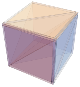
While the procedure is simple enough, the individual tetrahedrons were a bit difficult to visualize. To help with that, I’ve made a small Mathematica script that one can play with:
pts = {{-1, -1, -1}, {1, -1, -1}, {1, 1, -1}, {-1, 1, -1}, {-1, -1,
    1}, {1, -1, 1}, {1, 1, 1}, {-1, 1, 1}};
ti = {{1, 2, 6, 7}, {1, 2, 3, 7}, {1, 6, 7, 5}, {4, 1, 8, 7}, {1, 5,
   8, 7}, {1, 4, 3, 7}}; Graphics3D[{Opacity@0.4,
  Table[Tetrahedron[pts[[i]]], {i, ti}]}]
From that, we can easily see that mesh now.
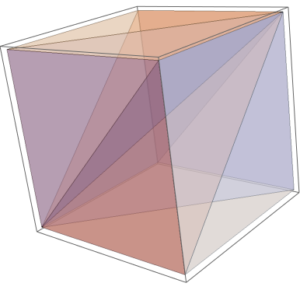
So what does the “conforming” part of the title mean? Of course, there is an easier way to tile the cube using only 5 tetrahedrons, but if you put together multiple cubes, one have to be careful of how you orient them. Using the above meshing, as long as the cubes are not too distorted and can easily create the tetrahedral mesh by drawing the diagonal in the same direction.
For example, below we have a eight hexahedral elements laid in a cube, but there are three slab, three columns, and two cubes (with one significantly smaller). This whole thing was needed so that I can construct something as anisotropic as the mesh below without resorting to fancy software.